Robust Fitting with Outliers

Replace a normal noise model with a Student-t model when a few observations are badly contaminated.

Source: Examples/Tutorials/RobustFittingWithOutliers.m

Switch the noise model from normal to Student-t

The workflow is the same as in the previous ConstrainedSpline tutorial, but now a few observations are badly contaminated. The key change is the distribution object: use a StudentTDistribution when you want the fit to be less sensitive to outliers than a normal model.

\[y_i = f(t_i) + \epsilon_i, \qquad \epsilon_i \sim t_{\nu}(0,\sigma).\]

rng(7)
t = linspace(0, 1, 60)';
xTrue = exp(-3*t).*sin(4*pi*t);
xObs = xTrue + 0.08*randn(size(t));
outlierIndex = [10 22 37 51];
xObs(outlierIndex) = xObs(outlierIndex) + [0.75; -0.55; 0.65; -0.70];
tq = linspace(t(1), t(end), 400)';

normalModel = NormalDistribution(sigma=0.08);
studentTModel = StudentTDistribution(sigma=0.08, nu=3);

normalFit = ConstrainedSpline.fromData(t, xObs, S=3, splineDOF=12, distribution=normalModel);
robustFit = ConstrainedSpline.fromData(t, xObs, S=3, splineDOF=12, distribution=studentTModel);

Plot the normal and Student-t fits on the same contaminated data.

figure(Position=[100 100 900 320])
plot(tq, exp(-3*tq).*sin(4*pi*tq), "k--", LineWidth=1.5), hold on
plot(tq, normalFit(tq), LineWidth=2)
plot(tq, robustFit(tq), LineWidth=2)
scatter(t, xObs, 28, "filled", MarkerFaceAlpha=0.65)
scatter(t(outlierIndex), xObs(outlierIndex), 72, "o", LineWidth=1.5)
xlabel("t")
ylabel("x(t)")
legend("Underlying signal", "Normal model", "Student-t model", "Observations", "Tagged outliers", Location="northeast")
grid on

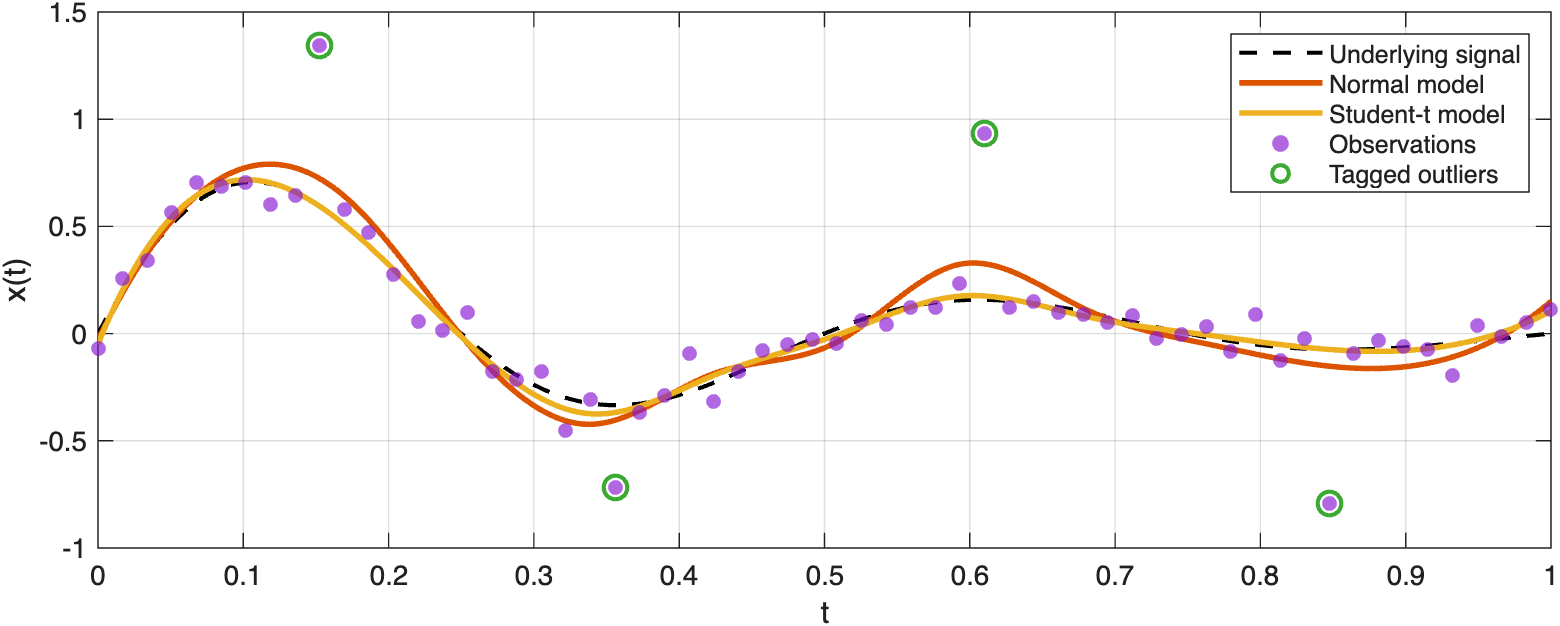
Changing the distribution from normal to Student-t makes the fit less sensitive to a few large outliers.

Inspect the final robust weights

Internally the robust fit is solved by an iteratively reweighted scheme, but the tutorial-level idea is simply that the Student-t model downweights observations that look much less plausible under a normal model. For the implementation details, see distribution and the developer topic tensorModelSolution.

Plot the final weights assigned by the robust fit.

figure(Position=[100 100 780 300])
stem(t, robustFit.W, "filled", LineWidth=1.2), hold on
scatter(t(outlierIndex), robustFit.W(outlierIndex), 70, "o", LineWidth=1.5)
xlabel("t")
ylabel("Final weight")
grid on

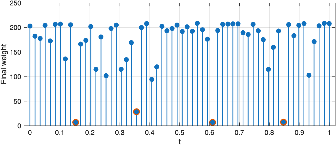
The final weights show which observations the Student-t fit decided to trust less.