BSpline Foundations

Build intuition for order, degree, knot placement, local support, and basis construction in one dimension.

Source: Examples/Tutorials/BSplineFoundations.m

Connect spline degree, order, and the basis expansion

The low-level one-dimensional BSpline model is

\[f(t)=\sum_{j=1}^{M}\xi_j B_{j,S}(t;\tau),\]

where S is the polynomial degree and the spline order is

\[K=S+1.\]

The easiest way to see the effect of S is to interpolate the same data with several choices of degree.

tData = 2*pi*2.5*[0; 1; 3; 4; 5; 8; 10]/10;
xData = sin(tData);

Plot the same interpolation problem for several spline degrees.

tq = linspace(tData(1), tData(end), 500)';
figure(Position=[100 100 960 640])
tiledlayout(2, 2, TileSpacing="compact")

for Splot = 0:3
    nexttile
    splineFit = InterpolatingSpline.fromGriddedValues(tData, xData, S=Splot);
    plot(tq, splineFit(tq), LineWidth=2), hold on
    scatter(tData, xData, 22, "filled")
    for knotValue = unique(splineFit.knotPoints(:)).'
        xline(knotValue, ":", Color=0.75*[1 1 1])
    end
    title(sprintf("S = %d, K = %d", Splot, Splot + 1))
    xlabel("t")
    ylabel("x(t)")
    grid on
end

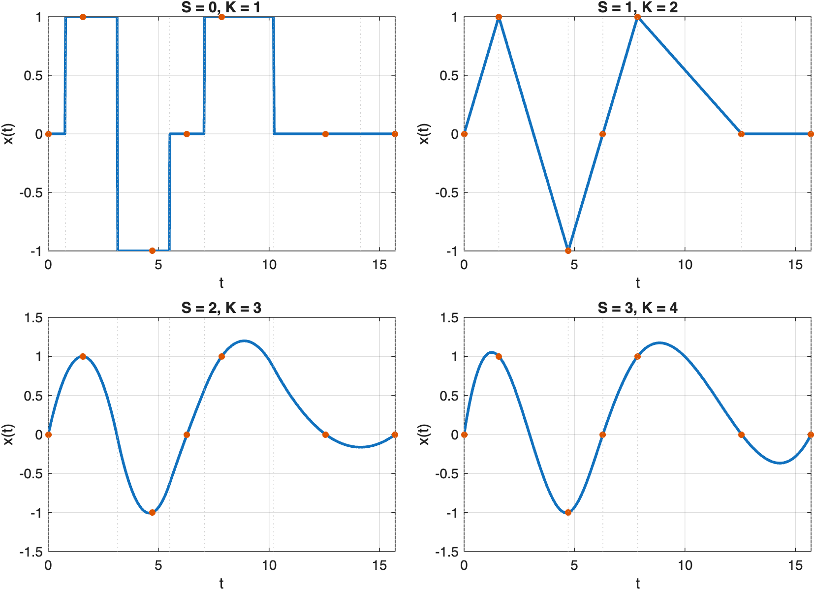
Increasing the spline degree raises the local polynomial order and the continuity between neighboring pieces.

Assemble the basis matrix explicitly

InterpolatingSpline hides the basis construction, but the public BSpline helpers expose the same steps directly: choose knot points with knotPointsForDataPoints, assemble the basis matrix with matrixForDataPoints, solve for the coefficients, and evaluate the resulting spline.

S = 3;
tq = linspace(tData(1), tData(end), 500)';

knotPoints = BSpline.knotPointsForDataPoints(tData, S=S);
basisMatrix = BSpline.matrixForDataPoints(tData, knotPoints=knotPoints, S=S);
xi = basisMatrix \ xData;

directSpline = BSpline(S=S, knotPoints=knotPoints, xi=xi);
interpolatingSpline = InterpolatingSpline.fromGriddedValues(tData, xData, S=S);

Plot the direct BSpline construction against InterpolatingSpline.

figure(Position=[100 100 820 320])
plot(tq, directSpline(tq), LineWidth=2), hold on
plot(tq, interpolatingSpline(tq), "--", LineWidth=1.5)
scatter(tData, xData, 28, "filled")
xlabel("t")
ylabel("x(t)")
legend("BSpline construction", "InterpolatingSpline", "Samples", Location="southoutside")
grid on

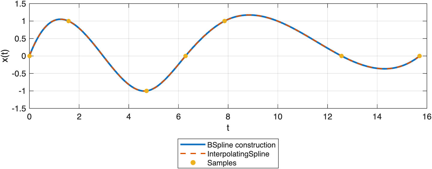
The low-level BSpline construction reproduces the same cubic interpolant as InterpolatingSpline when the same canonical knot sequence is used.

Repeated knots localize changes

Interior repeated knots reduce continuity and make the basis more local. That is useful when you want the spline to change behavior more sharply near a transition.

tqSupport = linspace(0, 4, 500)';
simpleKnots = [0; 0; 0; 0; 1; 2; 3; 4; 4; 4; 4];
repeatedKnots = [0; 0; 0; 0; 1; 2; 2; 3; 4; 4; 4; 4];

xiSimple = zeros(numel(simpleKnots) - 4, 1);
xiRepeated = zeros(numel(repeatedKnots) - 4, 1);
xiSimple(3) = 1;
xiRepeated(3) = 1;

simpleBasis = BSpline(S=3, knotPoints=simpleKnots, xi=xiSimple);
repeatedBasis = BSpline(S=3, knotPoints=repeatedKnots, xi=xiRepeated);

Plot one basis function with and without an interior repeated knot.

figure(Position=[100 100 820 320])
plot(tqSupport, simpleBasis(tqSupport), LineWidth=2), hold on
plot(tqSupport, repeatedBasis(tqSupport), LineWidth=2)
for knotValue = unique(repeatedBasis.knotPoints(:)).'
    xline(knotValue, ":", Color=0.75*[1 1 1])
end
xlabel("t")
ylabel("Basis value")
legend("Simple interior knots", "Repeated interior knot", Location="southoutside")
grid on

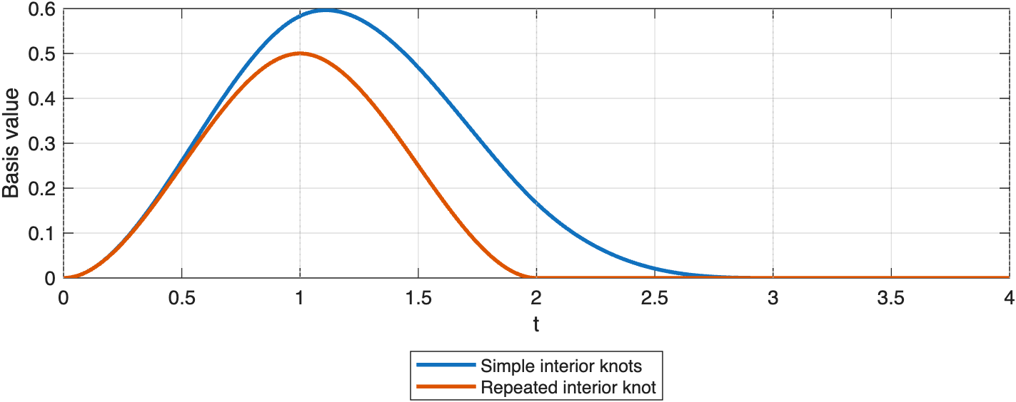
Repeating an interior knot makes the cubic basis function less smooth and more localized near that knot.