Spline Interpolation

Interpolate exact data in one dimension and on rectilinear grids, and compare the results with MATLAB’s griddedInterpolant.

Source: Examples/Tutorials/InterpolationOnGrids.m

Interpolate exact samples in one dimension

InterpolatingSpline is the shortest path from exact samples to a reusable spline object. Start with one irregular 1-D grid and evaluate the interpolant on a denser set of query points.

x = [0.00; 0.08; 0.21; 0.37; 0.55; 0.71; 0.86; 1.00];
y = exp(-1.6*x).*sin(2*pi*x);
xq = linspace(x(1), x(end), 400)';

spline1D = InterpolatingSpline.fromGriddedValues(x, y, S=3);
yq = spline1D(xq);

Plot the interpolant against the original samples.

figure(Position=[100 100 720 320])
plot(xq, yq, LineWidth=2), hold on
scatter(x, y, 42, "filled")
xlabel("x")
ylabel("f(x)")
legend("InterpolatingSpline", "Samples", Location="southoutside")
grid on

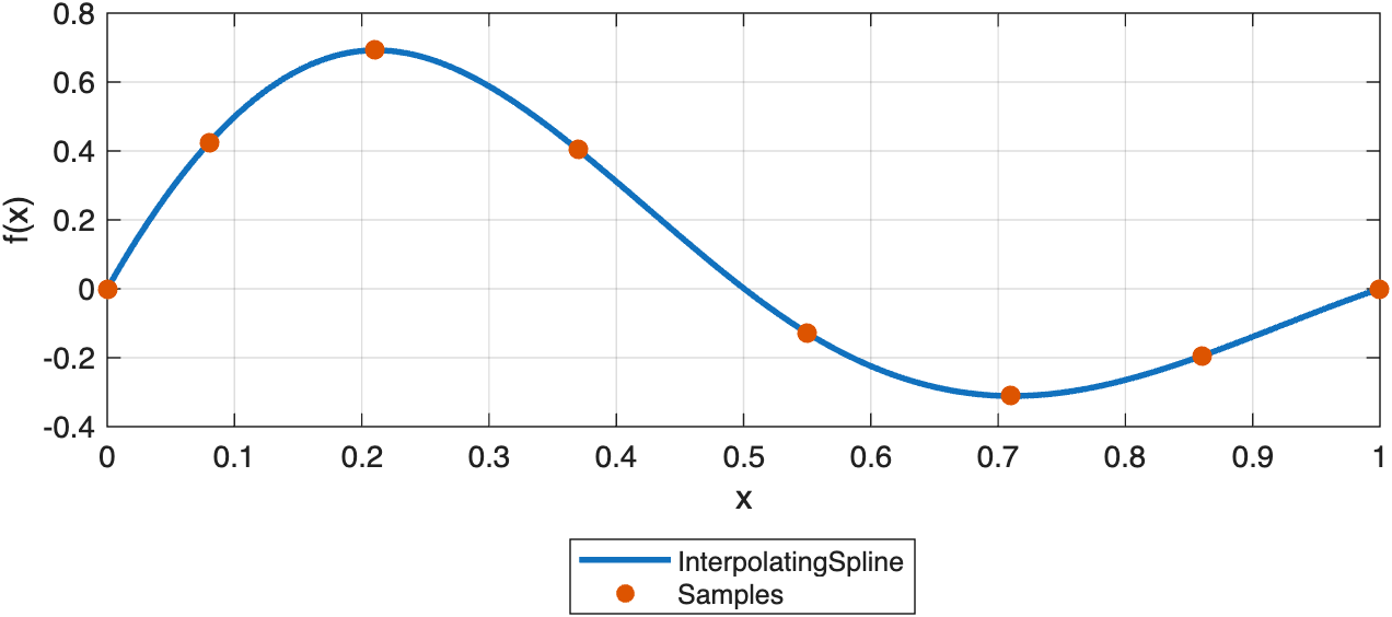
A one-dimensional InterpolatingSpline passes exactly through the supplied samples and can be evaluated on a denser grid.

Differentiate the same interpolant

Derivative evaluation uses the same spline object. In 1-D, set D=1 for the first derivative, D=2 for the second derivative, and so on.

dyq = spline1D.valueAtPoints(xq, D=1);

Plot the derivative on the same dense query grid.

figure(Position=[100 100 720 280])
plot(xq, dyq, LineWidth=2)
xlabel("x")
ylabel("df/dx")
grid on

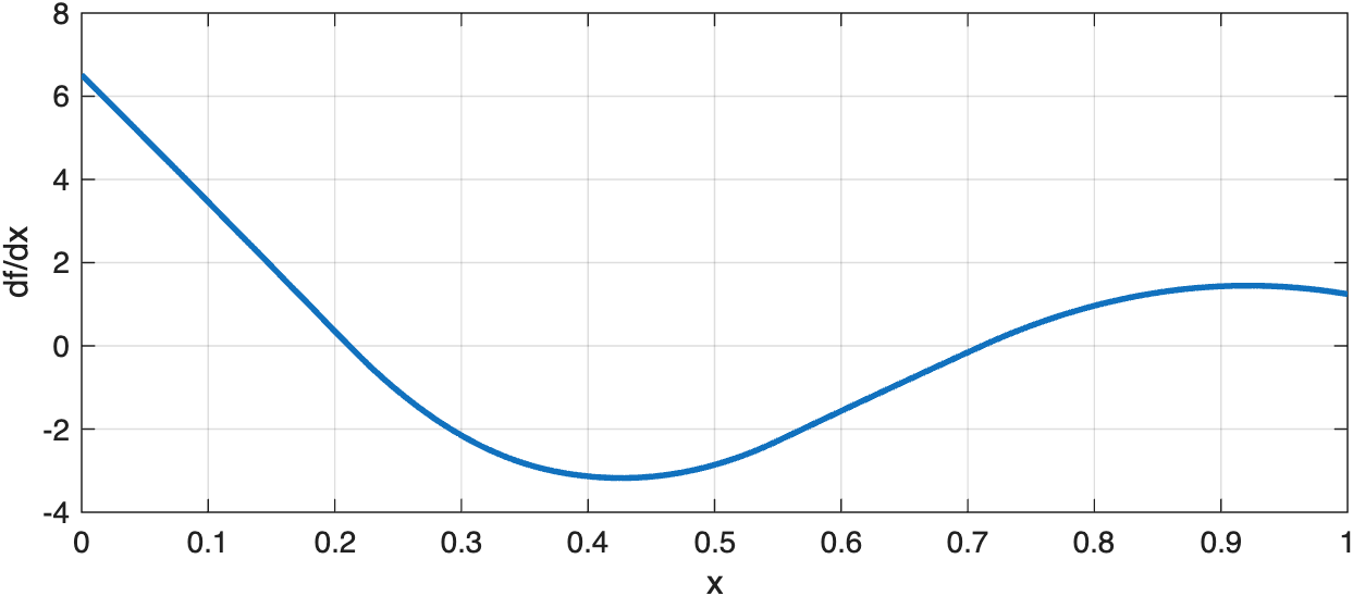
Derivative evaluation uses the same interpolant through valueAtPoints(…, D=1).

MATLAB’s closest built-in analogue here is griddedInterpolant. On this grid the values agree to machine precision, while InterpolatingSpline keeps the same spline-object workflow that the package uses everywhere else.

matlab1D = griddedInterpolant(x, y, "spline");
yqMatlab = matlab1D(xq);
maxDifference1D = max(abs(yq - yqMatlab));

Interpolate a rectilinear grid in two dimensions

The same constructor extends directly to tensor-product grids. Supply one coordinate vector per dimension together with the array of grid values.

xGrid = linspace(-1.2, 1.2, 9)';
yGrid = linspace(-1.5, 1.5, 11)';
[X, Y] = ndgrid(xGrid, yGrid);
F = cos(pi*X).*exp(-0.5*Y.^2) + 0.2*X.*Y;

xqGrid = linspace(xGrid(1), xGrid(end), 61)';
yqGrid = linspace(yGrid(1), yGrid(end), 71)';
[Xq, Yq] = ndgrid(xqGrid, yqGrid);

spline2D = InterpolatingSpline.fromGriddedValues({xGrid, yGrid}, F, S=[3 3]);
Fq = spline2D(Xq, Yq);

Plot the sampled grid beside the interpolated field.

figure(Position=[100 100 920 360])
tiledlayout(1, 2, TileSpacing="compact")

nexttile
imagesc(yGrid, xGrid, F)
axis xy
axis tight
colorbar
xlabel("y")
ylabel("x")
title("Sampled Grid")

nexttile
imagesc(yqGrid, xqGrid, Fq)
axis xy
axis tight
colorbar
xlabel("y")
ylabel("x")
title("Interpolated Grid")

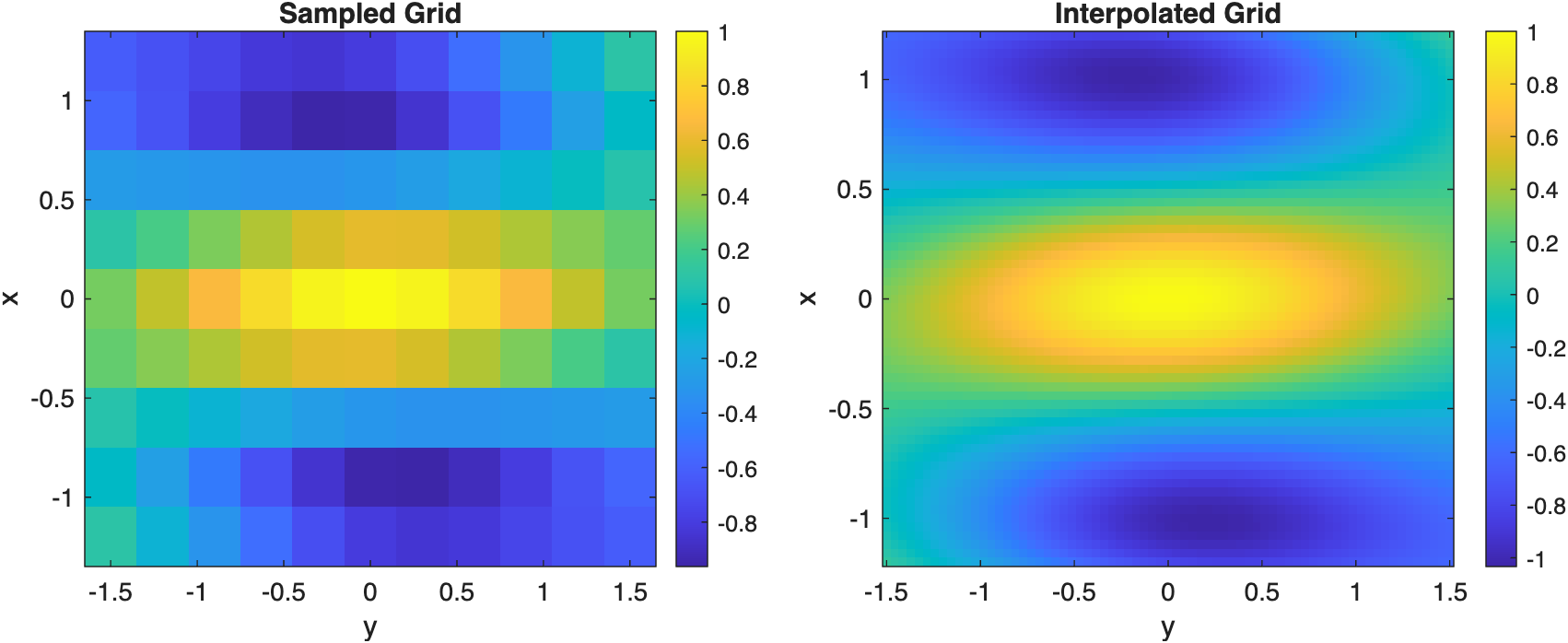
The same InterpolatingSpline workflow extends from one-dimensional data to rectilinear tensor grids.

griddedInterpolant is also the natural MATLAB comparison in two dimensions. On this rectilinear-grid problem the queried values again agree to machine precision.

matlab2D = griddedInterpolant({xGrid, yGrid}, F, "spline");
FqMatlab = matlab2D({xqGrid, yqGrid});
maxDifference2D = max(abs(Fq - FqMatlab), [], "all");