Internal Modes Basics

Initialize InternalModesSpectral, compute hydrostatic and fixed-frequency modes, and repeat the workflow for a realistic LatMix profile.

Source: Examples/Tutorials/InternalModesBasics.m

Initialize InternalModesSpectral from an exponential profile

This tutorial shows the minimum workflow for computing and plotting vertical modes with InternalModesSpectral. The same overall pattern also appears in InternalModesWKBSpectral, InternalModesAdaptiveSpectral, InternalModesDensitySpectral, and InternalModesFiniteDifference.

We start from the standard exponential stratification

\[N^2(z) = N_0^2 e^{2 z / b},\]

sample the implied density profile on a depth grid, and initialize the spectral solver on a denser output grid for plotting.

g = 9.81;
N0 = 5.2e-3;
b = 1300;

zIn = linspace(-5000, 0, 500).';
zOut = linspace(zIn(1), zIn(end), 1024).';
rho = 1025 * (1 + (b * N0^2 / (2 * g)) * (1 - exp(2 * zIn / b)));

im = InternalModesSpectral(rho=rho, zIn=zIn, zOut=zOut, latitude=33, nEVP=257);

Compute the hydrostatic modes

The simplest first solve is the hydrostatic call modesAtFrequency, which uses omega = 0 as the starting point.

[F, G] = im.modesAtFrequency(0);

figure(Color="w", Position=[100 100 980 360])
tiledlayout(1, 3, TileSpacing="compact", Padding="compact")

nexttile
plot(sqrt(im.N2), im.z, LineWidth=2)
xlabel("N(z) (rad s^{-1})")
ylabel("z (m)")
title("Exponential profile")
grid on

nexttile
plot(F(:, 1:4), im.z, LineWidth=1.5)
xlabel("F_j(z)")
title("Hydrostatic F modes")
grid on

nexttile
plot(G(:, 1:4), im.z, LineWidth=1.5)
xlabel("G_j(z)")
title("Hydrostatic G modes")
grid on

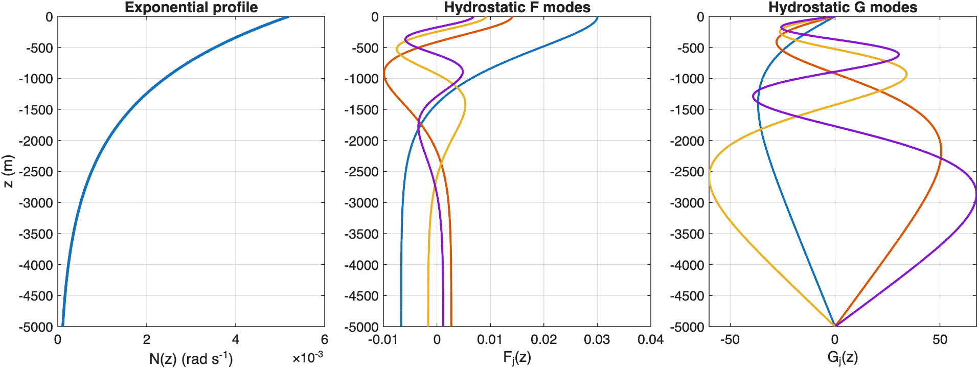
The hydrostatic solve gives a clean first look at the leading vertical modes for the standard exponential stratification.

Compute modes at a nonzero frequency

To move away from the hydrostatic limit, choose a representative frequency between f0 and the largest buoyancy frequency in the water column.

The companion fixed-wavenumber problem is also available through modesAtWavenumber, which returns [F, G, h, omega] for a chosen horizontal wavenumber k.

omega = im.f0 + 0.35 * (max(sqrt(im.N2)) - im.f0);
[F, G] = im.modesAtFrequency(omega);

figure(Color="w", Position=[100 100 980 360])
tiledlayout(1, 3, TileSpacing="compact", Padding="compact")

nexttile
plot(sqrt(im.N2), im.z, LineWidth=2)
xlabel("N(z) (rad s^{-1})")
ylabel("z (m)")
title("Exponential profile")
grid on

nexttile
plot(F(:, 1:4), im.z, LineWidth=1.5)
xlabel("F_j(z)")
title(sprintf("F modes at \\omega = %.2f f_0", omega / im.f0))
grid on

nexttile
plot(G(:, 1:4), im.z, LineWidth=1.5)
xlabel("G_j(z)")
title(sprintf("G modes at \\omega = %.2f f_0", omega / im.f0))
grid on

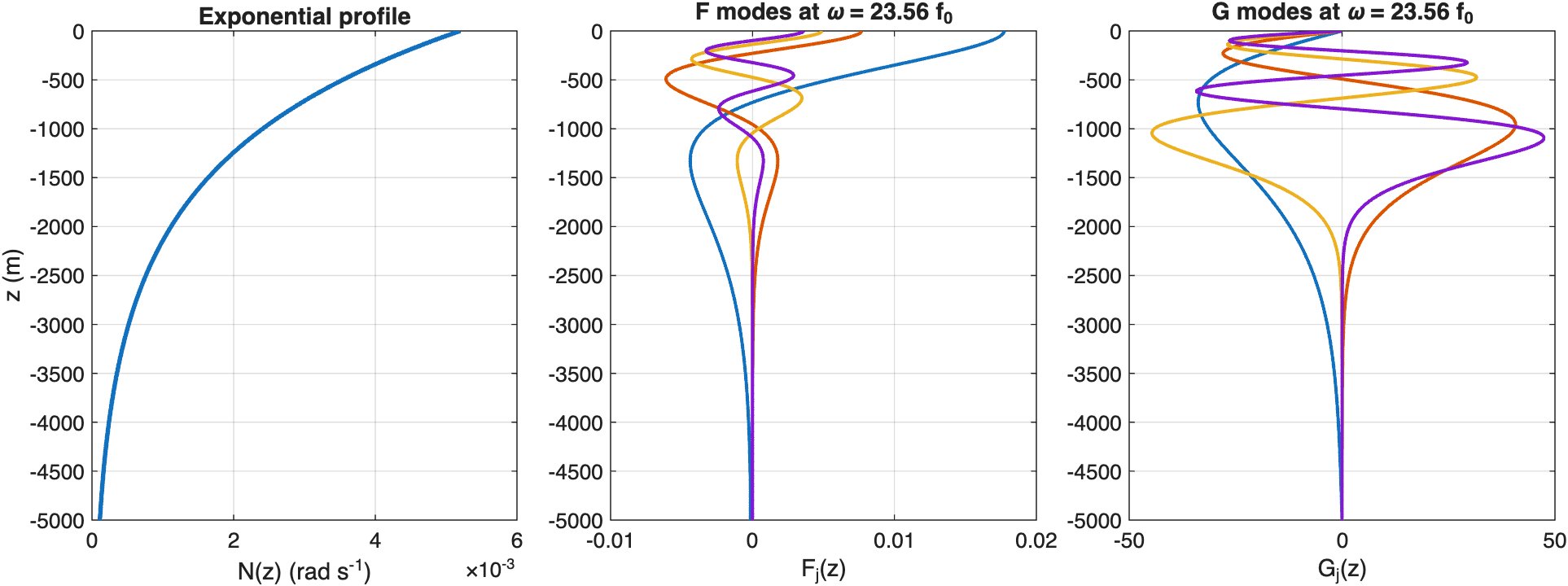
Choosing a nonzero frequency shifts the modal structure while keeping the same InternalModesSpectral workflow.

Compute modes for a realistic LatMix profile

The same solver can be initialized directly from a gridded observed profile. Here we load the first stored Site 1 LatMix profile that ships with the examples.

scriptDir = fileparts(mfilename("fullpath"));
latmixData = load(fullfile(scriptDir, "..", "SampleLatmixProfiles.mat"));

rhoLatMix = latmixData.rhoProfile{1};
zLatMix = latmixData.zProfile{1};
zOutLatMix = linspace(zLatMix(1), zLatMix(end), 1024).';

imLatMix = InternalModesSpectral(rho=rhoLatMix, zIn=zLatMix, zOut=zOutLatMix, latitude=latmixData.latitude, nEVP=257);
[F, G] = imLatMix.modesAtFrequency(0);

figure(Color="w", Position=[100 100 980 360])
tiledlayout(1, 3, TileSpacing="compact", Padding="compact")

nexttile
plot(imLatMix.rho, imLatMix.z, LineWidth=2)
xlabel("\rho(z) (kg m^{-3})")
ylabel("z (m)")
title("LatMix density profile")
grid on

nexttile
plot(F(:, 1:4), imLatMix.z, LineWidth=1.5)
xlabel("F_j(z)")
title("LatMix hydrostatic F modes")
grid on

nexttile
plot(G(:, 1:4), imLatMix.z, LineWidth=1.5)
xlabel("G_j(z)")
title("LatMix hydrostatic G modes")
grid on

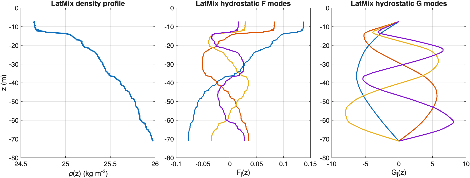
InternalModesSpectral works directly on the realistic LatMix profile and returns the leading hydrostatic modes on the requested output grid.

Choose the solver to match the profile

This LatMix density profile is not monotonic, so InternalModesWKBSpectral is not a good choice for this case. The depth-coordinate InternalModesSpectral solver still works directly on the supplied profile, which makes it a convenient default for realistic profiles like this one.